サンプルスクリプト
[1-1] 金属の溶解解析 【Melting.pde】

1. 概要

金属の溶解に対する FlexPDE の適用例を示します。システム変数として、温度を "temp"、固体材料の全ての断片を "Solid" とします。温度は、熱方程式によって与えられます。

	rho*cp*dt(temp) - div(lambda*grad(temp)) = Source

ここで、cp：熱容量
	rho：密度
	lambda：熱伝導率

潜熱（Qm）は、"Solid" が０から１へ変化する時に放出される全ての熱量です。
dH/dSolid = Qm（一定）と仮定して、
	Qm = integral[0,1]((dH/dSolid)*dSolid)

従って、凝固からの熱源は
	dH/dt = (dH/dSolid)*(dSolid/dt) = Qm*dt(Solid)

温度が（Tm-T0/2）から（Tm+T0/2）へ変化する時に、固体断片（Solid）が１から０への線形勾配で表
すことが出来ると仮定します。
	Solid = 1〔固体〕		temp < Tm-T0 の時
		(Tm+T0/2-temp)/T0	Tm-T0 <= temp <= Tm+T0 の時
		0〔液体〕		temp > Tm+T0 の時

ここで、Tm：融点温度
	T0：溶融遷移がそれ以上だと発生する温度範囲
この方程式に空間導関数がないので、ノイズ･フィルタの働きをするために小さな係数を持つ拡散項を導入し
ます。

ここで扱う問題は、液体(2000°)の槽に浸された冷えた固体材料(400°)のディスクです(解析モデルは断面です)。　初期段階はディスクに接した材料が凍るようなものです。　しかし、平衡状態に達すると、全ての材料は液体です。　外周境界は断熱されています。

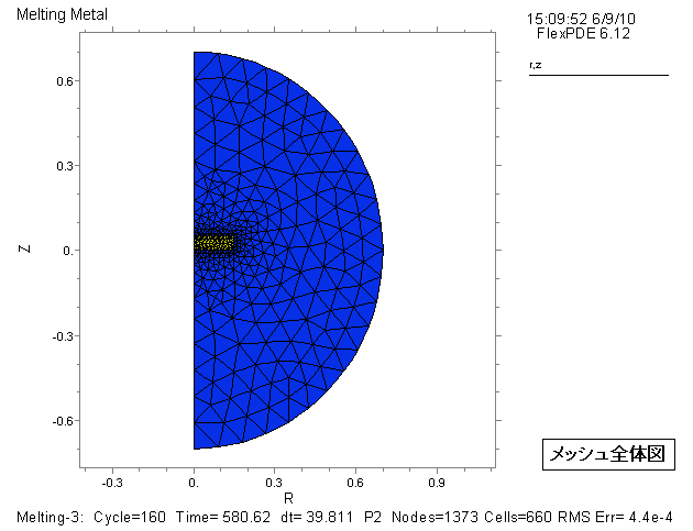
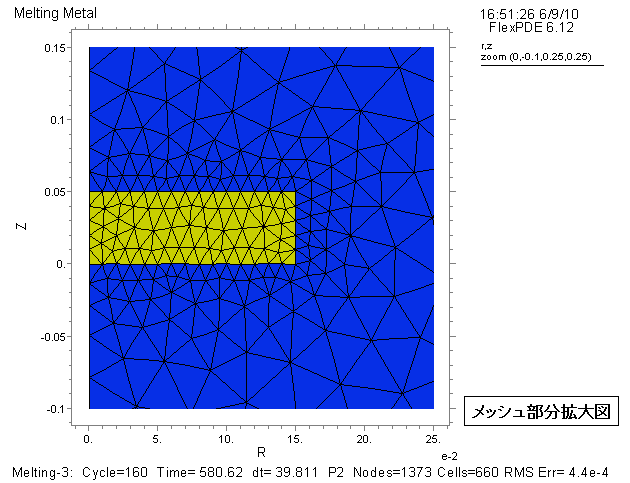
初期状態は不連続な分布なので、冷たい最初のディスクを定義するために別々のREGIONを使います。　そのため、メッシュの線はディスク形状に従います。　メッシュ全体図、部分拡大図をご参照下さい。　黄色が固体のディスク、青色が液体です。
メッシュ自動分割の急激な移行を助けるために、ディスクと境を接する特徴を加えます。　
"SELECT smoothinit"は、補間作用のオーバーシュートを最小にするのを助けます。

2. メッシュ図

3. 解析結果

温度分布図(全体図)、及び変数 Solid の時間変化（部分拡大図、Time=0, 1E-4, 1E-3, 1E-2, 0.1, 1, 10, 20, 30, 40, 50, 60, 70, 80, 90, 100, 200, 300, 600）を示します。　両者とも Time=300 で全体が液体に変化したことが読み取れます。
下図は FlexPDE から出力した、各時間ごとの状態を示す画像ファイルを Jasc Animation Shop 等の市販ソフトでアニメ.gifファイルへ変換しています。

{Fig.A}，{Fig.B} は、４項で対応するスクリプトを示します。
温度分布図 (全体図)：{Fig.A}

変数 Solid の時間変化 (部分拡大図)：{Fig.B}

4. スクリプト

下記のスクリプトをマウスでコピーし、FlexPDE エディット･ウィンドウに貼り付けて実行する際には、日本語のコメントを除去して下さい。　そのままですと、コンパイル･エラーが発生する場合があります｡

{  Melting.PDE

  This problem shows the application of FlexPDE to the melting of metal.

  We choose as our system variables the temperature, "temp", and the
  fraction of material which is solid at any point, "Solid".

  The temperature is given by the heat equation,

        rho*cp*dt(temp) - div(lambda*grad(temp)) = Source

  where cp is the heat capacity, rho the density and lambda the conductivity.

  The latent heat, Qm, is an amount of heat released as "Solid" changes from
  zero to one.   We have Qm = integral[0,1]((dH/dSolid)*dSolid), or assuming
  dH/dSolid is constant, dH/dSolid = Qm.
  Then heat source from freezing is

        dH/dt = (dH/dSolid)*(dSolid/dt) = Qm*dt(Solid).

  We assume that the solid fraction can be represented by a linear ramp from
  one down to zero as the temperature passes from (Tm-T0/2) to (Tm+T0/2).

        Solid = 1                   when  temp  <  Tm-T0
                (Tm+T0/2-temp)/T0   when  Tm-T0 <= temp <= Tm+T0
                0                   when  temp  >  Tm+T0

  where Tm is the melting temperature, and T0 is a temperature range over
  which the melting transition occurs.   Since there are no spatial
  derivatives in this equation, we introduce a diffusion term with small
  coefficient to act as a noise filter.

  The particular problem addressed here is a disk of cold solid material
  immersed in a bath of liquid.   The initial temperatures are such that
  material first freezes onto the disk, but after equilibrium is reached
  all the material is liquid.   The outer boundary is insulated.

  Since the initial condition is a discontinuous distribution, we use a separate
  REGION to define the cold initial disk, so that the grid lines will follow the
  shape.   We also add a FEATURE bounding the disk to help the gridder
  define the abrupt transition.   SELECT SMOOTHINIT helps minimize
  interpolator overshoots.
}

TITLE  'Melting Metal'

COORDINATES
  ycylinder('r','z')

SELECT
  smoothinit
  threads=2

VARIABLES
  temp(threshold=1)
  solid(threshold=0.01)

DEFINITIONS

  Qm= 225000        { latent heat：潜熱}
  Tm=1850           { Melting temperature：融点温度}
  T0= 20            { Melting interval +- T0：溶融遷移が発生する温度範囲}
  temp_liq=2000     { initial liquid temperature：最初の液体の温度}
  temp_sol=400      { initial solid temperature：最初の固体の温度}
  Tinit
  sinit

  R_inf = 0.7       { Domain Radius m：解析領域の半径}

  { plate }
  d=0.05
  dd = d/5          { a defining layer around discontinuity }
  R_Plate=0.15

  lambda = 30+4.5e-5*(temp-1350)^2 { Conductivity：熱伝導率}
  rho=2500                         { Density kg/m3：密度}
  cp = 700                         { heat capacity：熱容量}

INITIAL VALUES
  temp=Tinit
  solid =  0.5*erfc((tinit-Tm)/T0)

EQUATIONS
  temp:  rho*cp*dt(temp) - div(lambda*grad(temp)) = Qm*dt(solid)
  solid: solid - 1e-6*div(grad(solid)) = RAMP((temp-Tm), 1, 0, T0)

BOUNDARIES

  region 'Outer'
     Tinit = temp_liq
     sinit = 0
     start 'outer' (0,-R_inf)
       value(temp)= temp_liq    arc(center=0,0) angle 180
       natural(temp)=0          line to close

  region 'Plate'
     Tinit = temp_sol
     sinit = 1
     start(0,0)
       mesh_spacing=dd
       line to (R_Plate,0) to (R_Plate,d) to (0,d) to close

TIME  0 by 1e-5 to 600

MONITORS
 for cycle=10
   grid(r,z) zoom (0,-0.1,0.25,0.25)
   elevation(temp)  from(0.1,-0.1) to (0.1,0.15) range=(0,2000)
   elevation(solid) from(0.1,-0.1) to (0.1,0.15) range=(0,1)

PLOTS
   for t= 0 1e-4 1e-3 1e-2 0.1 1 10 by 10 to 100 by 100 to 300 by 300 to endtime
{ 時間 t=0, 1E-4, 1E-3, 1E-2, 0.1, 1, 10, 20, 30, 40, 50, 60, 70, 80, 90, 100,
  200, 300, 600 における下記の項目を出力します。　解析結果の該当画像を右クリック
  しますと、メニューが表示されて時間結果を変更できます。
}
   contour(temp)  painted  range=(0,2000)				{Fig.A}
   contour(temp)    zoom (0,-0.2,0.45,0.45) range=(0,2000)
   elevation(temp)  from(0.1,-0.1) to (0.1,0.15) range=(0,2000)
   contour(solid)   range=(0,1)
   contour(solid)   zoom (0,-0.2,0.45,0.45) range=(0,1)
   surface(solid)   zoom (0,-0.2,0.45,0.45) range=(0,1) viewpoint(1,-1,30) {Fig.B}
   elevation(solid) from(0.1,-0.1) to (0.1,0.15) range=(0,1)

HISTORIES

   history(temp)  at (0.051,d/2) at (0.075,d/2) at (R_plate,d/2)
   history(temp)  at (0.051,d)   at (0.075,d)   at (R_plate,d)
   history(solid) at (0.051,d/2) at (0.075,d/2) at (R_plate,d/2)
   history(solid) at (0.051,d)   at (0.075,d)   at (R_plate,d)
   history(integral(cp*temp+Qm*(1-solid))) as "Total Energy"

END